Hidden Markov Model for Trading Using Python

Hello, my name is Lubomyr and today we will talk about Hidden Markov Model

or HHM. Maybe you have heard about this model before or you are hearing about it for the first time. I will tell you what this model is, where it is used and how to apply it in trading So…

1. What is Hidden Markov Model?

Hidden Markov Models (HMMs) are powerful statistical tools with applications ranging from speech recognition to financial modeling. In this article, I will explore what HMMs are, their uses, and how they can be applied to stock market trading, along with code examples and visualizations.

A Hidden Markov Model (HMM) is a type of Markov model where the observations depend on an underlying, unobservable (hidden) Markov process, often denoted as X. In an HMM, there exists an observable process Y, whose outcomes are influenced by the hidden states of X in a defined way. Since the hidden states of X cannot be directly observed, the primary objective is to infer the state of X by analyzing the outcomes of Y.

By definition, an HMM adheres to the Markov property, which requires that the outcome of Y at any time t depends only on the corresponding state of X at the same time t. Additionally, the past states and observations (i.e., for times prior to t) must be conditionally independent of Y at time t, given the state of X at that time.

To estimate the parameters of an HMM, maximum likelihood estimation is commonly used. For linear chain HMMs, the Baum–Welch algorithm is a standard method for parameter estimation.

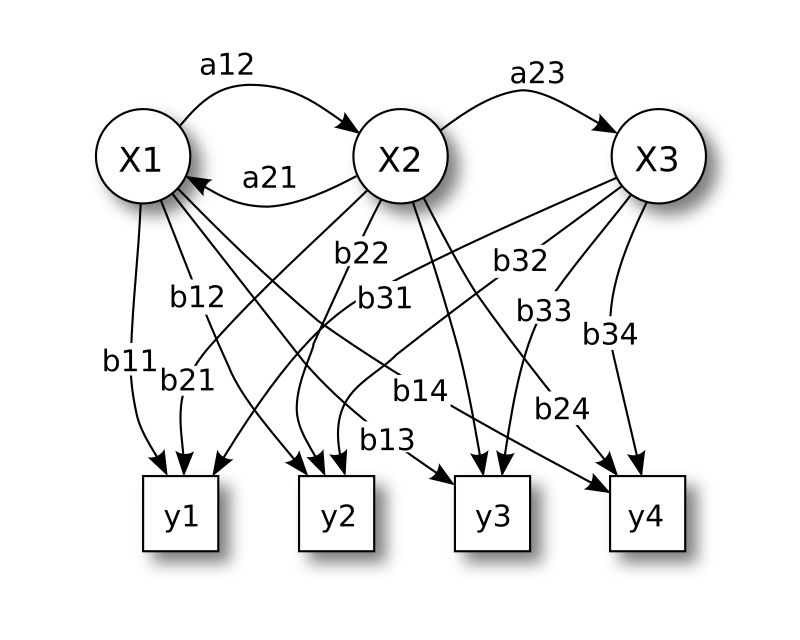
In its discrete form, a hidden Markov process can be thought of as an extension of the urn problem with replacement, where each item is returned to the original urn before the next draw. Imagine a scenario where a genie operates in a hidden room, inaccessible to an observer. The room contains several urns—labeled as X1, X2, X3, and so on—each filled with a known mixture of uniquely labeled balls, such as y1, y2, y3, etc.

The genie selects an urn at random and draws a ball from it, placing the ball onto a conveyor belt visible to the observer. However, the observer can only see the sequence of balls on the conveyor belt, not the sequence of urns the genie used. The genie follows a rule for selecting urns, where the choice of urn for the current ball depends solely on a random number and the urn used for the previous ball. The selection process does not depend on urns chosen earlier than the most recent one, making this a Markov process. This concept is represented in the upper portion of Figure 1.

Since the Markov process—the sequence of urns—cannot be directly observed, and only the labeled balls are visible, this setup is referred to as a hidden Markov process. The lower portion of Figure 1 illustrates this arrangement, showing that balls like y1, y2, y3, and y4 can be drawn at each state. Even if the observer knows the composition of the urns and observes a sequence of three balls (e.g., y1, y2, and y3) on the conveyor belt, they cannot determine with certainty which urn the third ball was drawn from. However, the observer can calculate other useful information, such as the probability that the third ball came from a specific urn.

Also more about model you can read here

2. For What Can You Use the Hidden Markov Model?

HMMs have a wide range of applications, including:

Speech and Voice Recognition: Understanding spoken words based on audio signals.
Natural Language Processing: Part-of-speech tagging and machine translation.
Bioinformatics: Analyzing DNA sequences and predicting protein structures.
Anomaly Detection: Identifying fraud or unusual patterns in datasets.
Financial Modeling: Modeling market regimes and stock price movements.

In this article, we’ll focus on using HMMs in the context of stock market trading.

3. How to install HMM?

pip install hmmlearn

4. Examples of HMM Code

To demonstrate HMMs, let’s start with a basic example using Python. Here, we’ll use the hmmlearn library to train an HMM on sample data:

import numpy as np from hmmlearn import hmm # Example: Three hidden states with Gaussian emissions model = hmm.GaussianHMM(n_components=3, covariance_type="diag", n_iter=100, random_state=42) # Sample data: sequence of observed values X = np.random.rand(100, 1) # 100 samples, 1 feature # Fit the model to the data model.fit(X) # Predict hidden states hidden_states = model.predict(X) print("Hidden States:", hidden_states)

This code trains a basic HMM with three hidden states on a random dataset. The hidden_states variable contains the inferred states for each observation.

4. How to Use HMM in Stock Market Trading

Stock prices often exhibit patterns influenced by underlying market conditions, such as bullish or bearish trends. HMMs can help identify these hidden market regimes by analyzing historical price and indicator data.

In stock trading, HMMs can:

Detect Market Regimes: Classify periods as bullish, bearish, or neutral.
Predict Trends: Use hidden states to anticipate price movements.
Optimize Strategies: Combine with trading indicators (e.g., RSI, MACD) to make informed decisions.

5. Example Code for HMM in Stock Trading

Here’s a practical example of applying HMM to analyze market trends using historical price data:

import pandas as pd
import numpy as np
from hmmlearn import hmm
from sklearn.preprocessing import StandardScaler
import psycopg2

# Database connection and data retrieval
symbol = 'ETHUSDT'
connection = psycopg2.connect(
    f"user='{config.postgre_user}' host='{config.postgre_host}'

password='{config.postgre_password}'

port='{config.postgre_port}'"
)
cursor = connection.cursor()

postgres_select_query = """ SELECT close, open, high, low, value, rsi, macd
                            FROM trading_coin_values
                            WHERE symbol = %s
                            ORDER BY id DESC
                            LIMIT 3000"""
cursor.execute(postgres_select_query, (symbol,))
data = cursor.fetchall()

# Prepare the data
df = pd.DataFrame(data, columns=['close', 'open', 'high', 'low', 'value', 'rsi', 'macd']).dropna()
scaler = StandardScaler()
X_scaled = scaler.fit_transform(df)

# Train the HMM
n_states = 3
model = hmm.GaussianHMM(n_components=n_states, covariance_type="diag", n_iter=500, random_state=42)
model.fit(X_scaled)

# Predict hidden states
df['hidden_state'] = model.predict(X_scaled)
print(df[['close', 'hidden_state']].tail())

This is a simple use of the HMM model. We can also add the ability to train the model, which will speed it up and help us get more accurate results.

# Select relevant features
features = df[['close', 'open', 'high', 'low', 'value', 'rsi', 'macd']].dropna()

# Normalize the features
scaler = StandardScaler()
X_scaled = scaler.fit_transform(features.values)

# Split the data into 80% training and 20% testing
train_size = int(len(X_scaled) * 0.8)  # Calculate the training size
X_train = X_scaled[:train_size]        # First 80% of the data
X_test = X_scaled[train_size:]         # Last 20% of the data

# Train the HMM model
n_states = 3  # Adjust the number of hidden states as needed
model = hmm.GaussianHMM(
    n_components=n_states,
    covariance_type="diag",
    n_iter=500,
    random_state=42,
    init_params='cm'  # Prevent overwriting custom startprob_ and transmat_
)

# Initialize the start probabilities and transition matrix
model.startprob_ = np.full(n_states, 1 / n_states)  # Equal probabilities
model.transmat_ = np.full((n_states, n_states), 1 / n_states)  # Equal transition probabilities

# Fit the model on the training data
model.fit(X_train)

# Predict hidden states for the test set
hidden_states_train = model.predict(X_train)
hidden_states_test = model.predict(X_test)
hidden_states = np.concatenate([hidden_states_train, hidden_states_test])
df['hidden_state'] = hidden_states
# Analyze hidden states in the test set
df_train = df.iloc[:train_size].copy()
df_test = df.iloc[train_size:].copy()
df_train['hidden_state'] = hidden_states_train
df_test['hidden_state'] = hidden_states_test

Also, based on this data, we can decide whether to buy now, sell, or hold.

last_hidden_state = df_test['hidden_state'].iloc[-1]
if last_hidden_state == 0:
    print("Market is likely bullish; consider buying.")
elif last_hidden_state == 1:
    print("Market is likely bearish; consider selling.")
else:
    print("Market is neutral; hold position.")

Here is a result base on my ETHUSDT data

As you can see, in this situation it is better to hold on to your assets.

6. How to Plot HMM Results

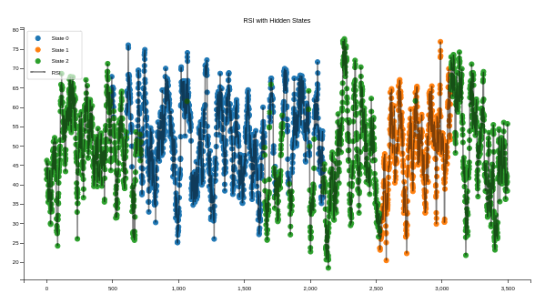
Visualizing the results can help you better understand the hidden states and their relationship to market indicators. Below is an example of plotting the Relative Strength Index (RSI) with hidden states:

Code is:

plt.figure(figsize=(12, 6))
for state in range(n_states):
    state_data = df[df['hidden_state'] == state]
    plt.scatter(state_data.index, state_data['rsi'], label=f'State {state}')
plt.plot(df['rsi'], color='black', alpha=0.5, label='RSI')
plt.legend()
plt.title("RSI with Hidden States")
plt.show()

Result is:

This code produces a scatter plot of RSI values color-coded by hidden state, with a translucent red line showing the overall RSI trend.

Conclusion

Hidden Markov Models offer a unique approach to uncovering hidden patterns in stock market data. By identifying market regimes and trends, traders can make more informed decisions. While HMMs have limitations—such as assumptions of linearity and normality—they remain a valuable tool for statistical modeling in finance.

Stay tuned for more in-depth articles about applying machine learning to trading!

Also read:
Mastering Hidden Markov Models for Algorithmic Trading: A Comprehensive Guide

Nine types of programmers in 2024

Meilisearch - organizing search in conjunction with Laravel

Advanced use of forms in Django using the example of Bootstrap and crispy

What a developer should never do

Images of Dell Inspiron 14 7441 Plus and XPS 13 9345 laptops have appeared